Heap Sort

Heap sort uses the heap data structure to sort an array. A heap is a complete binary tree, where each node is less than or equal to its parent. The binary tree below is a heap, because each parent node is greater than or equal to both of its child nodes.

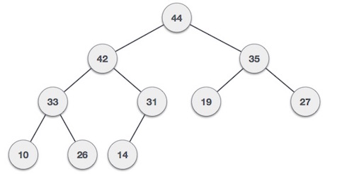
Heaps can be represented as arrays, where the position of each array element corresponds to its position in the binary tree. Tree nodes are labeled from top to bottom, and left to right. For example, the third element of the heap pictured above is 35.

We can represent a heap in Python as a list. Because the heap is a binary tree, the position of the parent node is related to the position of its children. The children nodes of any parent can be found using the index of the parent. If the parent has index \(i\), the left and right children can be found at indices \(2i + 1\) and \(2i + 2\).

Convince yourself of this using the code below.

A = [44, 42, 35, 33, 31, 19, 27, 10, 26, 14]

parent = 2
left = 2*parent + 1
right = 2*parent + 2

"""
A[parent] = 35
A[left] = 19
A[right] = 27
"""

Heapify

The first algorithm we will build, as part of heapsort, is the heapify algorithm. Heapify floats a node which is out of place, down the heap. The two child trees of the selected node must both be heaps, in order for heapify to work.

Inspect the binary tree below, and you will see that node 2, which has a value of 26, violates the heap property, since its value is less than the values of its children. Let’s build an algorithm to float 26 down so that the binary tree becomes a heap.

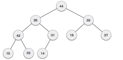
Remember the above binary tree can be represented as an array.

A = [44, 26, 35, 42, 31, 19, 27, 10, 33, 14]

Heapify will move an out-of-place node down the tree by comparing it to its children. If the selection is greater than the children, heapify will exchange the selection with the child. The algorithm iterates down the tree using a recursive call onto itself.

The following is an implementation of the heapify algorithm, as defined in Introduction to Algorithms.

def heapify(binary_tree: list, parent: int) -> list:
    ###
    # 1 - computation
    ###

    left = 2*parent + 1
    right = 2*parent + 2

    if(left <= len(binary_tree) - 1) and (binary_tree[left] > binary_tree[parent]):
        largest = left
    else:
        largest = parent

    if(right <= len(binary_tree) - 1) and (binary_tree[right] > binary_tree[largest]):
        largest = right

    if(largest != parent):
        tmp = binary_tree[parent]
        binary_tree[parent] = binary_tree[largest]
        binary_tree[largest] = tmp

    ###
    # 2 - recursion
    ###
        heapify(binary_tree, largest)

    return binary_tree

The heapify function has two steps - a computation, and a recursive call to itself. The computation has constant runtime, since accessing the length of an array and accessing an element of the array are both lookups. It can be shown that the upper bound on the recursion is \(T(2n/3)\). Combine the two, and we get the upper bound on the execution time of heapify.

Soving for the recursion, we get

Heap Build

Heapify can be used to construct a heap from an unsorted array. In order for the heapify algorithm to work, the child trees both need to be heaps. So, we need to apply heapify in a bottom up manner so that the child trees are guaranteed to be heaps before heapify is run at a node.

The last element of a binary tree with children, has \(n/2\) cardinality. We don’t need to run the algorithm on the set of nodes with no children, since these nodes are already one-element heaps. So, we only need to call heapify in reverse order, on the set of elements with children.

def build_heap(input_array: list) -> list:
    """Builds a heap from an unordered array.
    """
    i = len(input_array) // 2 - 1

    while(i >= 0):
        input_array = heapify(input_array, i)

        print(input_array)
        i = i - 1

    return input_array

Starting with the \(A[n/2]\) element, we will call heapify \(n/2\) times. Therefore, the upper bound on the execution time of heap build is the product of \(n/2\) and the execution time of heapify.

In most contexts we can neglect the constant factor and simplify.

Using some clever math, we can further simplify the upper bound.

Heap Sort

Heaps can be used to generate sorted arrays. After all, we are still building a sorting algorithm! In a heap, the maximum element will be stored at the root node. The first element of the heap will become the last element of the sorted array, if the array is sorted in ascending order.

If we remove the first element of the heap, we need to replace it with another element. What if we replaced it with the last element of the heap, so that we swapped the first and last elements of the heap? The root node of the heap would violate the heap property, but all other nodes would be heap-like. Therefore, we only need to call heapify to float the out-of-place element down the heap!

In this manner we can reduce the size of the heap by replacing the first element, reducing the size of the heap, and calling heapify to restore the heap. Ater \((n-1)\) iterations, we will reduce the size of the heap to 0.

def heap_sort(input_array: list) -> list:
    """Sorts an input array in ascending order.
    """
    heap = build_heap(input_array)

    i = len(heap) - 1

    while(i >= 0):
        tmp = heap[0]
        heap[0] = heap[i]
        heap[i] = tmp

        i = i - 1

        heap = heapify(heap, i, 0)

    return heap

Notice that this algorithm sorts in place - the data structure which is created, tmp in the code below, is of constant size. The call to build_heap makes one call to build_heap, and \(n - 1\) calls to heapify. The upper bound on heap_sort can be shown to be