Bicycles and Cold Weather

Are people less likely to ride bicycles during a stint of cold weather? This analysis sets out to answer that question, using a data from the Capital Bikeshare system in Washington DC. The operators of the Capital Bikeshare system have published their system data for research, and we are going to use a small sample of that data collected during 2011 and 2012. The dataset is available on the UCI website.

The hourly datset includes 17,379 observations, representing approximately 8760 hourly observations recorded over a 2 year period. Each observation records the timestamp, normalized temperature and a count of total rental bikes. I will focus on these features to keep our model simple.

My hypothesis is that temperature can be used to predict the count of rental bikes. When the temperature increases, the count of rental bikes will also increase. This hypothesis is motivated by my own experience as a bike rider who does not particularly enjoy biking in cold weather.

Linear Model

I will use a linear Bayesian model to represent the relationship between an observed temperature \(t_i\), and and observed bike count \(x_i\). Notice that each of our parameters is defined as a stochastic distribution - this is a feature of Bayesian analyses. The only parameter which is not defined as a distribution is \(\mu\), and that is because \(\mu\) is defined entirely in terms of other stochastic parameters.

\[x_i \sim Normal(\mu, \sigma) \\ \mu = \alpha + \beta (t_i - \bar t) \\ \alpha \sim Normal(400,100) \\ \beta \sim Normal(0, 100) \\ \sigma \sim Uniform(0, 200)\]

Likelihood

The first equation in the model is the likelihood function - it is the probability of the data \(x_i\), given our prior beliefs. I constructed the likelihood function as a normal distribution, because I did not have a good reason to use a different type of distribution.

\[x_i \sim Normal(\mu, \sigma)\]

As Richard McElreath points out in his book Statistical Rethinking, the normal distribution is a good first order approximation to many stochastic processes because of the central limit theorem, which states that observations of independent random variables tend towards a normal distribution.

Our likelihood function is defined by two parameters, the mean \(\mu\) and the variance \(\sigma\). The parameters \(\mu\) and \(\sigma\) are not observed, and we will need to construct a prior belief about their distribution. First, let’s define \(\mu\) in terms of the other observable parameter, temperature. This relation is our linear model.

\[\mu = \alpha + \beta (t_i - \bar t )\]

Now we have three unobserved parameters (\(\alpha, \beta, \sigma\)), in addition to our three observable parameters (\(x_i, t_i, \bar t\)). Notice I did not include \(\mu\) in the list of unobserved parameters, because \(\mu\) is a joint distribution, completely defined by the other parameters.

Priors

Let’s construct prior distributions for each of the unobserved parameters. This step requires some intuition, so we will think it through. The plots are generated using code which I have uploaded to Github.

A good place to start is by thinking about extreme values. When the observed temperature \(t_i\) equals the average observed temperature \(\bar t\), the equation for \(\mu\) will simplify.

\[\mu = \alpha + \beta (t_i - \bar t) \\ \mu = \alpha + \beta (0) \\ \mu = \alpha\]

When the observed temperature equals the average temperature, I expect the bike count to fall in the middle of the observed range. The bike counts range from 1 to 1000, so I am going to define \(\alpha\) as a normal distribution, centered around 400.

\[\alpha \sim Normal(400,200)\]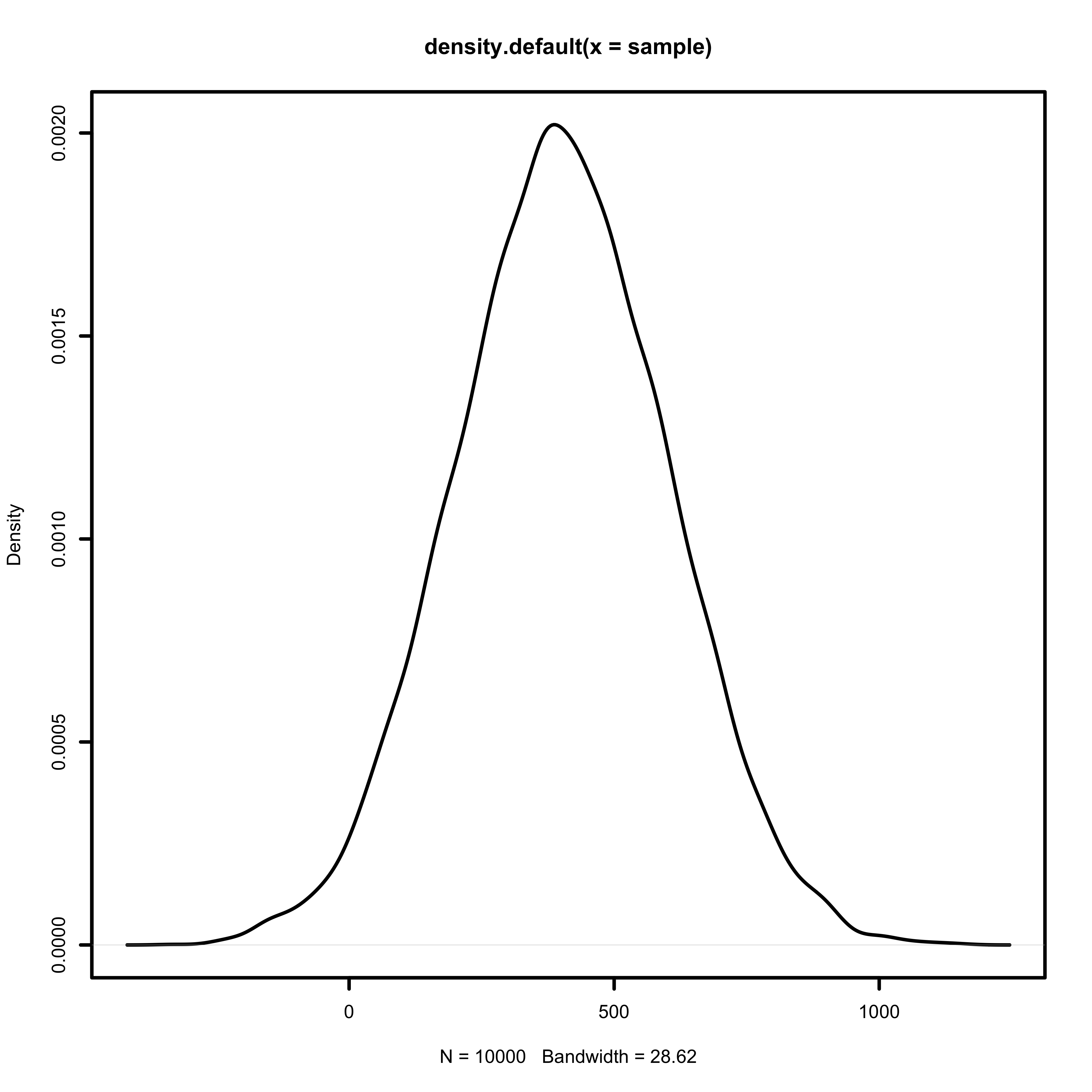

Let’s try to understand the rate of change between normalized temperature \(t_i\) and bike counts \(x_i\). The maximum temperature ever recorded in Washington D.C. is 41 Celsius, and the minimum is -21 Celsius. This gives us a maximum range of 62 Celsius. The normalized temperature ranges from 0 to 1. One-tenth the normalized temperature range represents approximately 6.2 degrees.

Let’s take a look at rate of change of our linear equation. Suppose a 6.2 degree difference resulted in 100 additional riders.

\[\Delta x_i = \beta \Delta t_i \\ 100 = \beta (0.1) \\ 1000 = \beta\]

We will take a more conservative estimate, and define \(\beta\) as a normal distribution centered around 500, with a variance of 200.

\[\beta \sim Normal(500, 200)\]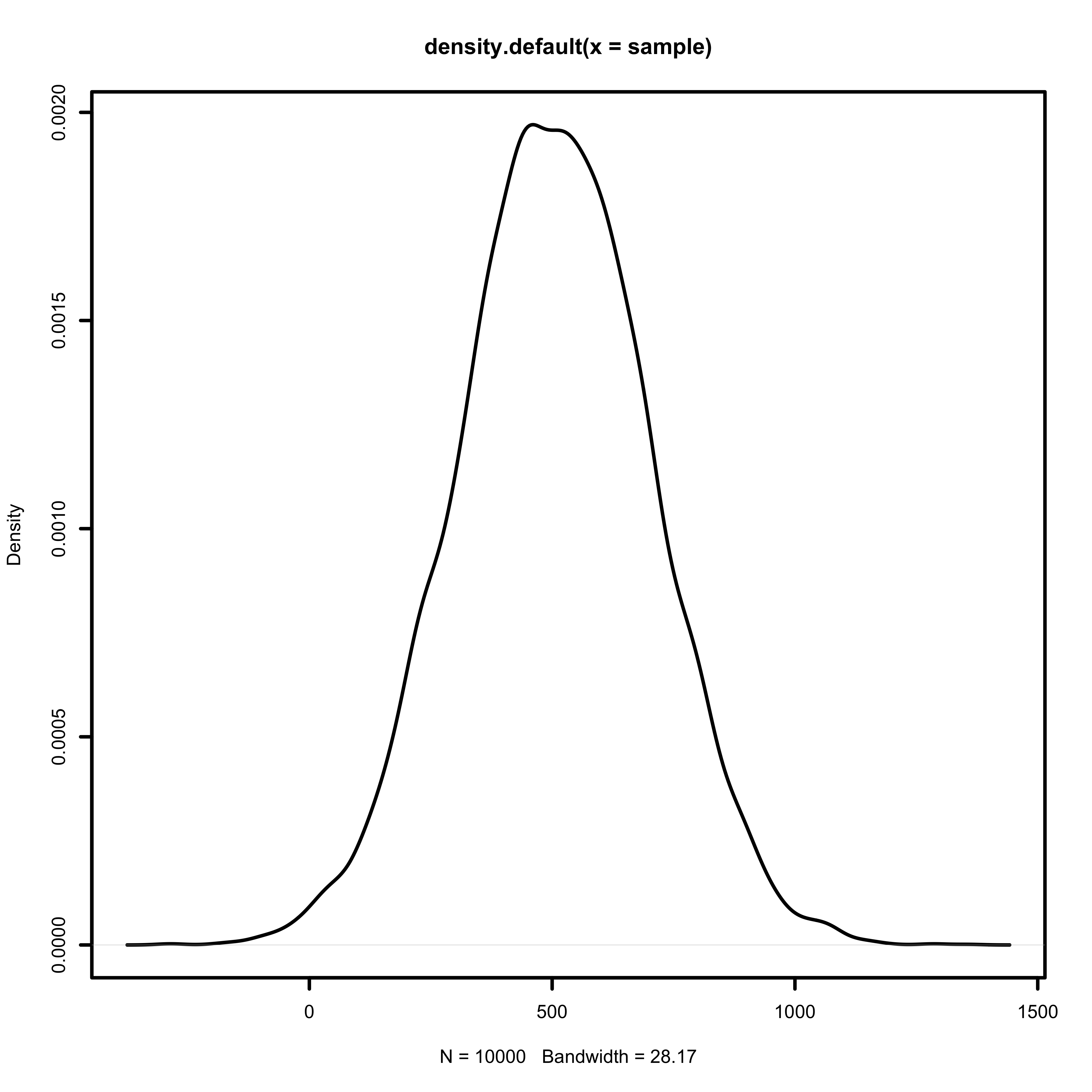

Finally, we need to construct a prior for the variance of the likelihood function. Variance must be positive, so we can once again bound it at zero. Recall that our bike counts range from 1 to 1000. I will use a uniform distribution between 0 and 200 as the initial prior, so that the mean plus or minus 2 standard deviations covers 80% of the observed range of bike counts.

\[\sigma \sim Uniform(0, 200)\]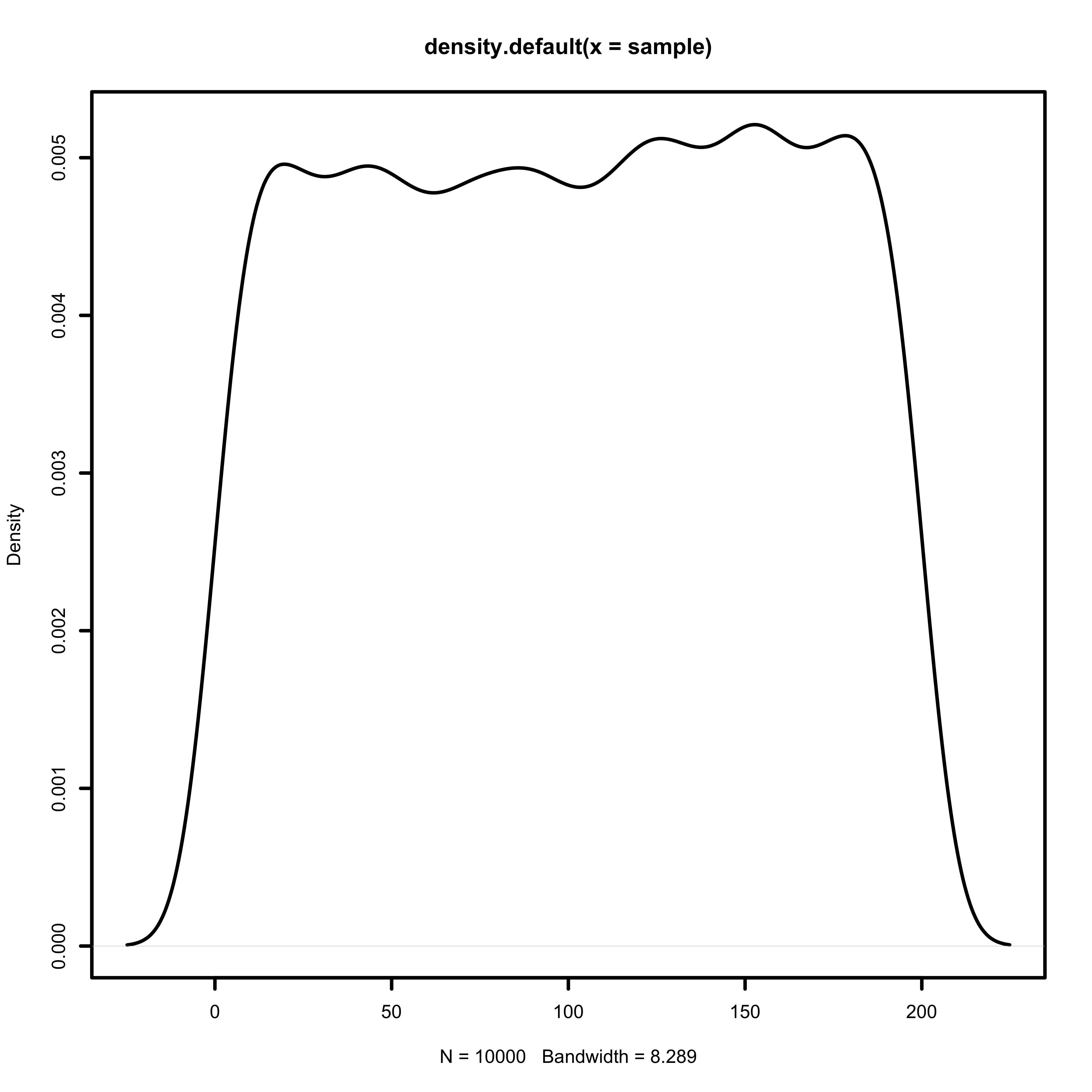

Prior Prediction

Now let’s sample from the likelihood function, and see how our model predicts bike counts. To produce the prior prediction, I will take 100 samples from \(\alpha\) and \(\beta\), substitute the observed mean in the dataset for \(\bar t\), and plot each of the 100 lines which are predicted by our likelihood function. The R code to produce this plot can be found on Github.

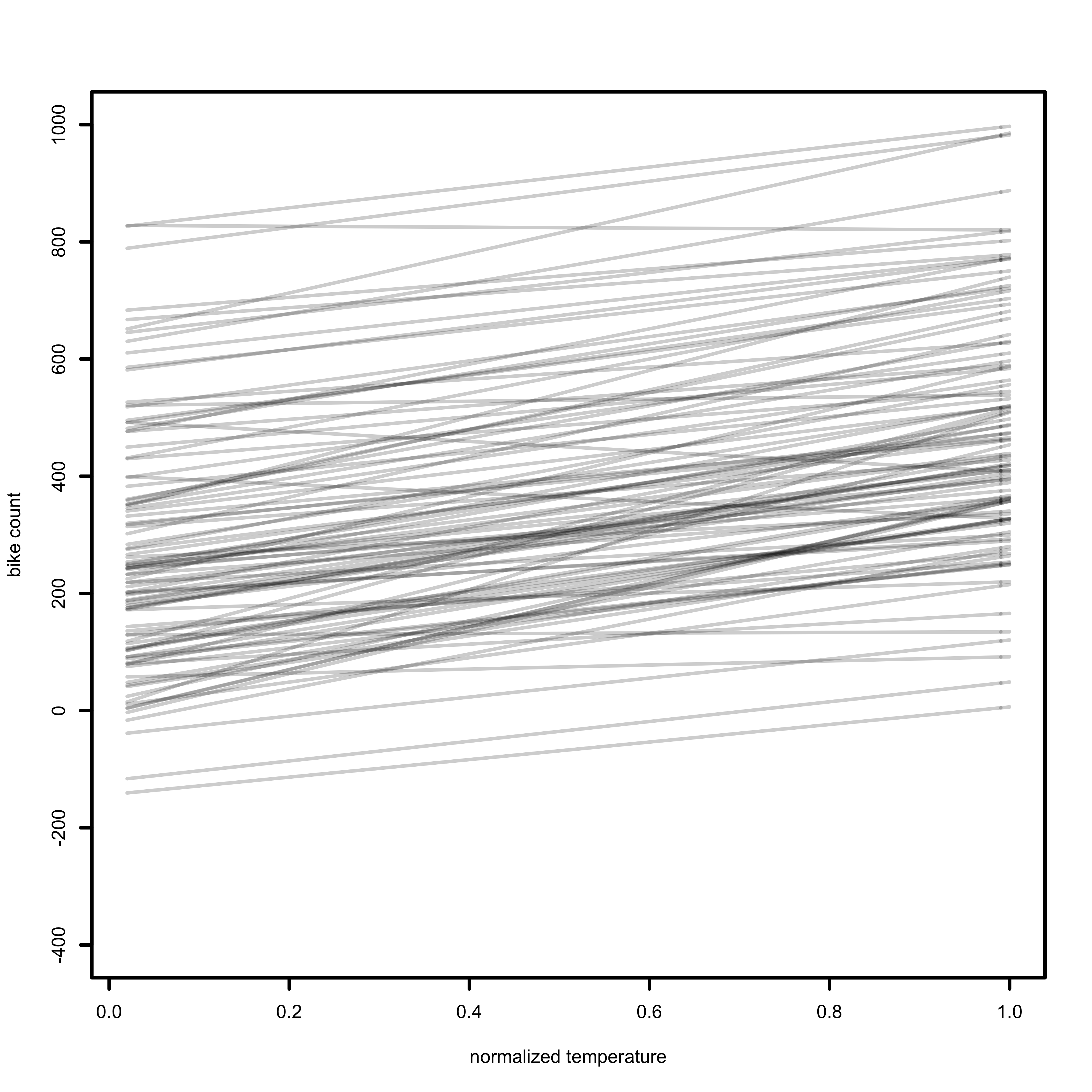
Our prior prediction does cover the range of the observed values from 1 to 1000. It could certainly be improved by eliminating the priors which predict negative values for \(x_i\), since negative bike counts are impossible. For now, we will accept the weaknesses of our priors and move on to the next step of our analysis.

Posterior Distribution

I will use the quadratic approximation to find the posterior distribution. The quadratic approximation approximates the posterior as a Gaussian distribution, and finds the peak and curvature near the peak.

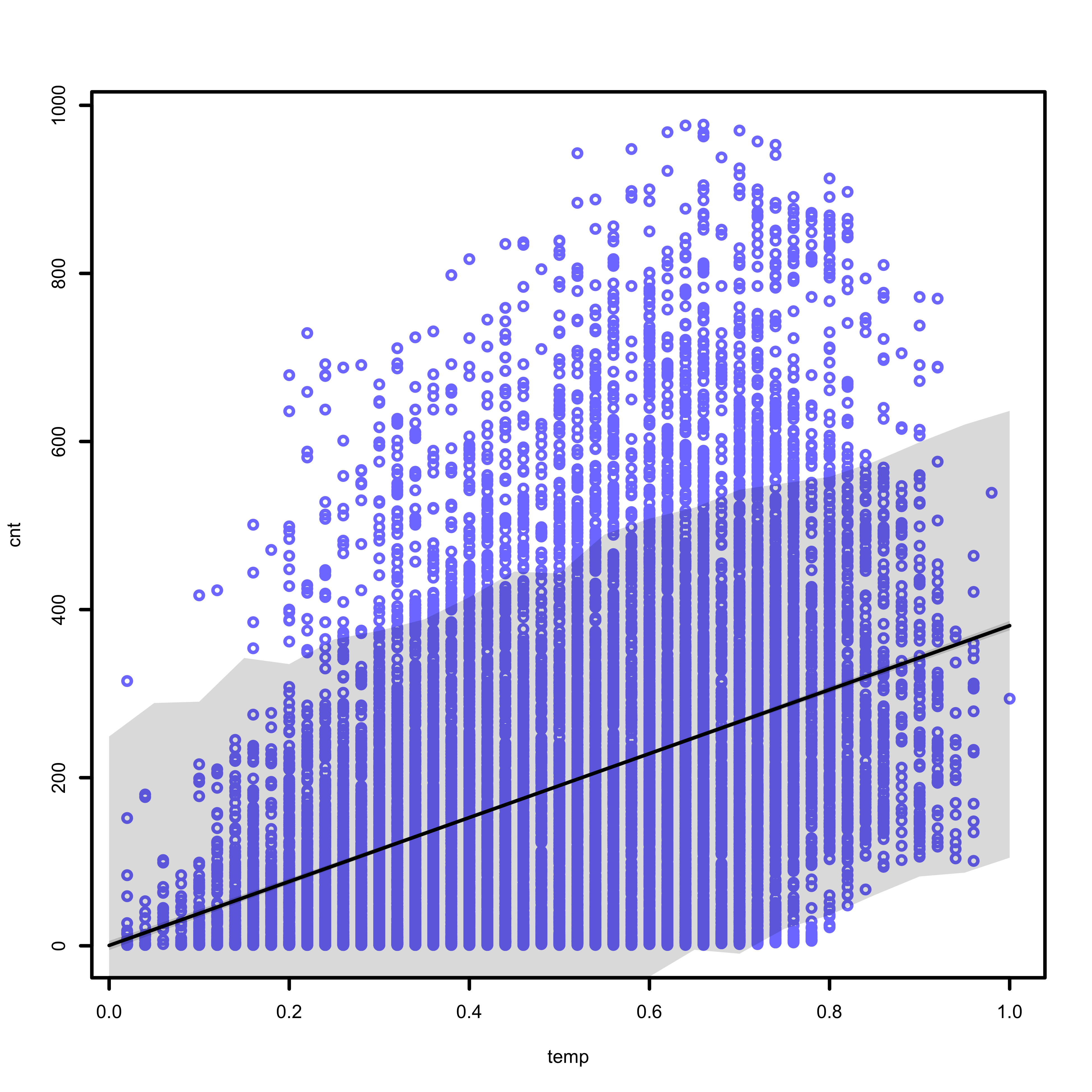
The figure below displays several different pieces of information. The blue points represent the observed data, collected by the Capital Bikeshare System. The solid black line represents the average predicted count, at each temperature value. The shaded region represents the 89% prediction interval, calculated at each temperature value.

The code which generates this plot can be found on Github.

Model Evaluation

Our model is entirely deficient in some ways, and useful in other ways. The first weakness of the model is its failure to describe bike counts about 600. The 89% prediction interval does not include the largest bike counts, and fails to describe a large portion of the data.

The model does do a good job describing the lower bound of bike counts when it is warm outside. The 89% prediction interval excludes the bottom right of the graph, which represents low bike counts when the temperature is high. The data also does not include any values in this region, which indicates that our model accurately represents this aspect of the data we have collected. Of course, the sample we collected may not represent the world at large.

By examining the data, it is apparent that a linear model may not describe the data. An exponential or higher order polynomial may do a better job describing the data. Future analyses could explore the predictions of a polynomial model in this context.