Weighted Coin Flip
Let’s do a simple Bayesian analysis of a weighted coin flip. For the purposes of the experiment, suppose you are having dinner with your friends, and one of your friends brings a coin. Your friend suggests a game - she will flip a coin 100 times, and the person who predicts the number of heads most accurately wins.
Prior
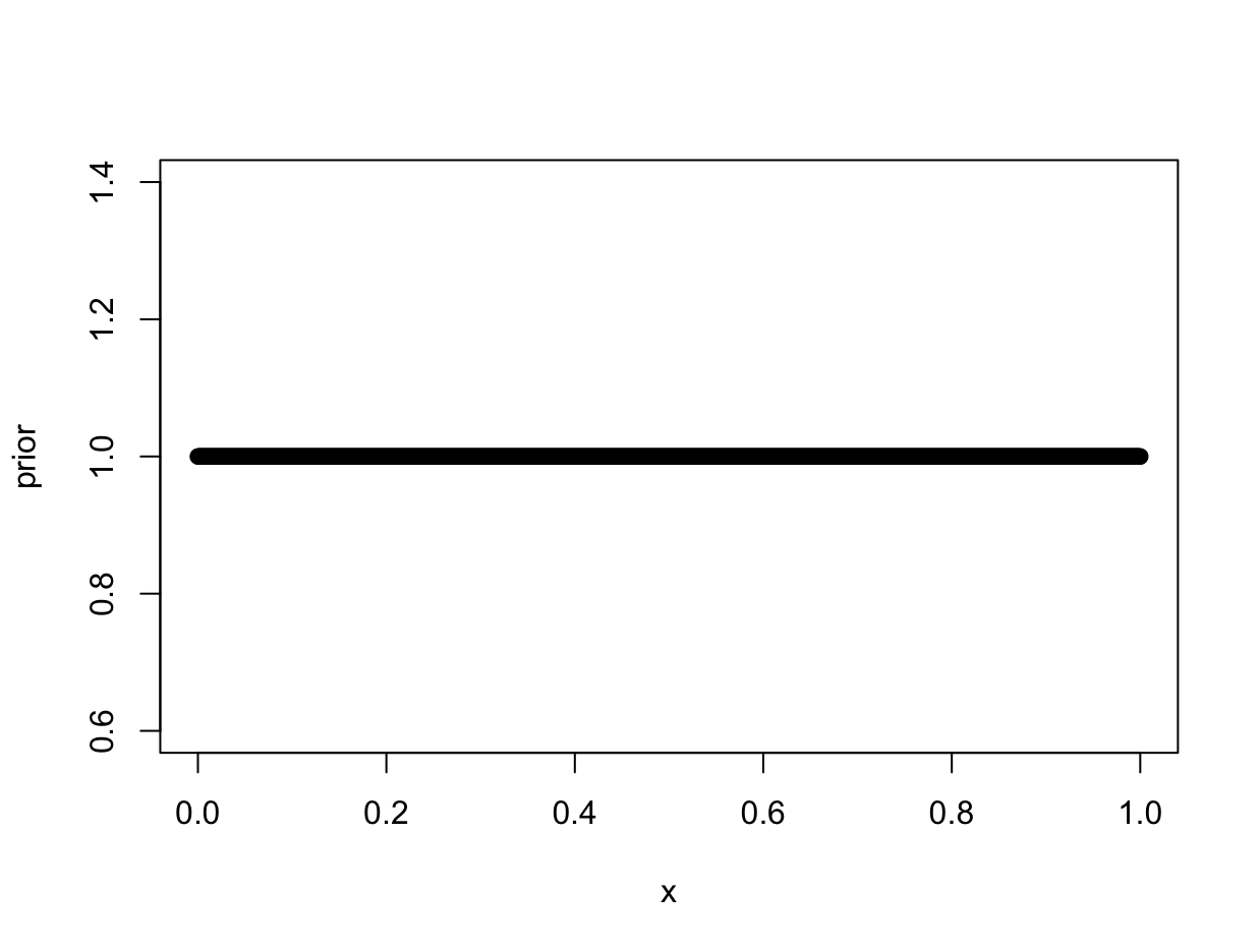
This particular friend is known to be shady. You suspect that the coin is not a fair coin. You suspect the coin is weighted, but you don’t have a good reason to suspect it is weighted towards heads rather than tails. The prior is therefore a uniform distribution - each of the probabilities has an equal likelihood of being true.
x <- seq( from=0 , to=1 , length.out=1000 )
prior <- rep( 1 , 1000 )
plot(x, prior)
Likelihood
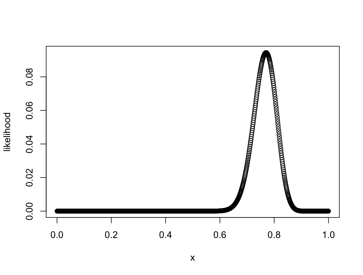
Your friend flips the coin, and out of 100 coin flips, 77 are heads. This is the experiment data, and we can use it to update the prior. In Bayesian analyis, we use the experiment data to compute the likelihood of each prior prediction. Essentially, we are using data to update our model of the world.
Let’s use a grid analysis to perform a numerical analysis. First, instantiate a vector with 1000 evenly-spaced values between 0 and 1, to represent the probability p of the coin landing on heads. Then, compute the likelihood of that value of p, using the binomial probability mass function. Note in the code below that since we pass a vector into dbinom(), the result is also computed as a vector.
p_grid <- seq( from=0 , to=1 , length.out=1000 )
likelihood <- dbinom( 77 , size=100 , prob=p_grid )
Posterior
Now we can compute the posterior distribution. In Bayesian analysis, the posterior distribution is the prior distribution multiplied by the likelihood of the data. Since the prior is a uniform distribution, our posterior will be identical to our likelihood function.
posterior <- likelihood * prior
plot(x, posterior)

Sampling the Posterior
In our case, the posterior distribution has an analytic solution (at this point the posterior can be represented by the binomial probability mass function, since the posterior was formed by multiplying a uniform prior and the likelihood). However, in more complex Bayesian models, the posterior does not have a simple solution. It can be computatationally expensive to even calculate the posterior distribution. In this case we can approximate the posterior distribution by sampling it.
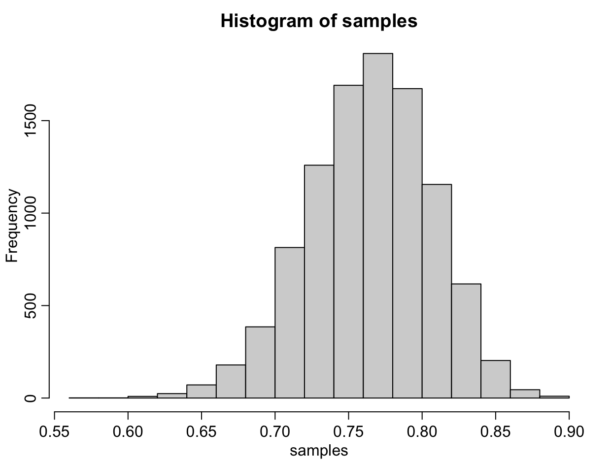
Let’s take 10,000 samples from the posterior distribution. We are sampling the values of the parameter p, which represents the probability that the coin will land on heads. Recall the vector p_grid represents 1000 discrete parameter values, and the vector posterior represents the plausability of each parameter value.
samples <- sample( p_grid , prob=posterior , size=1e4 , replace=TRUE )
hist(samples)
Each value in the samples vector is one of the discrete parameter values specified in p_grid. Let’s create a histogram of the samples drawn from the posterior distribution.
Interpreting the Model
The posterior distribution gives us the likelihood of different parameter values. If we were to predict the results of the next 100 coin flips, we could use the posterior distribution to select a parameter value to use in our calculations. In this simple experiment, the most likely parameter value is 0.77, as the posterior distribution is entirely formed by the data (recall the prior was a uniform distribution).
There are definite limitations to our model. The model assumes independence between events, but we know that the physical world is deterministic and a past flip of the coin could influence future coin flips. In his book Statistical Rethinking, Richard McElreath points out that physical events are deterministic and therefore past events can influence future events. This could inspire a debate on free will but for our purposes, suffice it to say that the assumption of independence is questionable.
The prior distribution could also be improved. Physics makes it extremely unlikely that the coin would have a 99% probability of landing on heads. Extreme parameter values are unlikely, but our prior distribution treats 0.99 and 0.70 as equally plausible.
The next time your friend wants to play the game, you can use your posterior distribution to make a prediction! After the game, you can use the new experiment data to update the model. The current posterior would become your new prior, and it can be updated using new experiment data.