Binomial Distribution

The binomial distribution measures the number of successes in an experiment which has two possible outcomes. Flipping a coin is a binomial experiment - the experiment can produce one of two values, H or T. We can define the two outcomes as success and failure, depending on the context. Mathematically, the probability of X successes, given a likelihood p and number of experiments x can be expressed like so:

The binomial distribution assumes independence between each experiment. Let’s plot P(x), for 7 coin flips. In this case x represents the number of successes in our experiment. We can use P(x) to compute the probability of each outcome - in this case, there are only 7 possible outcomes. First, initialize an array to represent the discrete values of x.

x <- 0:100

Now, compute the array of probabilities for each outcome.

y <- dbinom(x, size=100, prob=0.5)

Plot x against y to see the probability mass function.

plot(x, y, type='h')

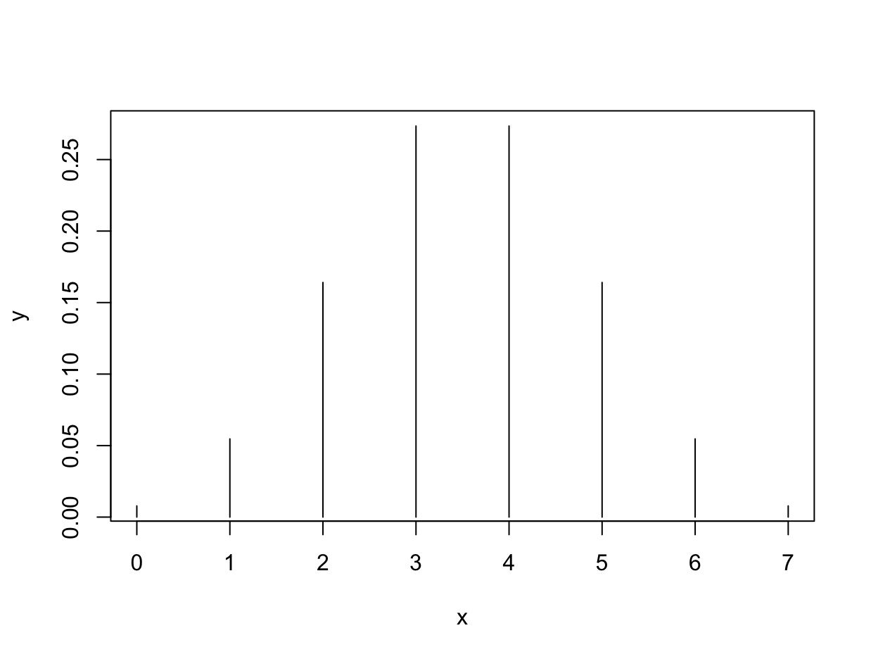
Note the pdf is normalized, if you add up each P(x), the values will sum to 1. The binomial distribution can be used to define the likelihood of an outcome. The likelihood is used to update the prior, in Bayesian statistics.