Quick Sort

Quick sort uses recursion to break the unsorted array into smaller subarrays, each of which is sorted before recombining the sorted subarrays into a complete sorted array. This approach to problem solving is described as the divide-and-conquer paradigm in CLRS.

The first step of the algorithm partitions the unsorted array into two subarrays. Each element of the left subarray is less than or equal to each element in the right subarray. The partitioning step selects a pivot element, which is the boundary between the two subarrays. Elements less than the pivot are placed in the left subarray, and elements greater than the pivot are placed in the right subarray.

def partition(A: list, p: int, r: int) -> int:
    """Partitions an array into two subarrays.
    """
    x = A[p]

    i = p - 1
    j = r + 1

    while True:
        i = i + 1
        j = j - 1

        while(A[j] > x):
            j = j - 1
        while(A[i] < x):
            i = i + 1

        if(i < j):
            A[i], A[j] = A[j], A[i]
        else:
            break

    return j

Notice in the code above that the while loop executes until the indices i and j cross. The loop will iterate through each element in the array A. If we define \(n\) as the number of elements in array A, the partition function has \(\theta (n)\) runtime.

Quick sort makes recursive calls to the partition function to sort the input array.

def quick_sort(A: list, p: int, r: int) -> list:
    """Sorts an unsorted array.
    """
    if(p < r):
        q = partition(A, p, r)

        quick_sort(A, p, q)
        quick_sort(A, q+1, r)

Runtime

Let’s first consider the upper bound on the runtime of quick sort. If each partition creates a subarray with one element and another subarray with \(n-1\) elements, the number of recursions will be maximal. The recursion tree below demonstrates the worst-case partitioning scenario.

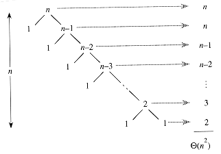
The execution time of each level of the recursion tree is defined by the number of elements in the partition. Remember that we found the runtime of the partition function to be \(\theta (n)\). To get the total runtime of the recursion tree above, we only need to sum the runtime of each recursive step.

The arithmetic series has solution \(\frac{1}{2} n(n+1)\). Neglecting the constants and coefficients, we arrive at the conclusion that the worst-case runtime is \(n^2\).

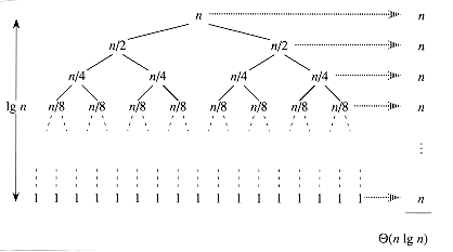
What about the best-case runtime? The number of recursions will be minimal when the partitioning is perfectly balanced at each depth of the recursion tree. Consider the recursion tree below, which has a depth of \(\log n\). Since the runtime of each recursion is \(\theta (n)\), the total runtime is \(T(n) = n \log n\).

More useful than the worst-case and best-case runtime is the average runtime. Consider an unbalanced partitioning scheme which places \(1/10\) of the elements in the left partition and \(9/10\) in the right partition. It can be shown that this recursion tree also has a depth of \(\log n\). The runtime of each recursion is, at most, \(\theta (n)\). Therefore the runtime of this unbalanced partitioning scheme is bounded by